Combining reports and exports - XLOOKUP
Picqer offers various reports and exports. Sometimes you may want to combine data from two exports. You can do this using the XLOOKUP formula, the modern replacement for VLOOKUP.
XLOOKUP
With the XLOOKUP formula in Excel, you can add data from one table to another, as long as at least one field matches.
The formula explained
For this example, we have exported 2 files. Table 1 which contains productcodes and names, and table 2 which contains productcodes, suppliers, and prices. We want to combine these 2 files and add the price of a product (from table 2) to table 1. This way, we end up with 1 table containing productcode, name, and price.
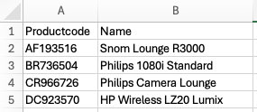 Table 1
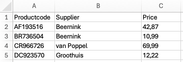 Table 2
The XLOOKUP formula looks like this:
=XLOOKUP(lookup_value, lookup_array, return_array, [if_not_found],[match_mode],[search_mode])
As you can see, the productcode is included in both files. We can use this field to link the data in both tables. In table 1 we will be adding the formula in cell C2, in order to add the price to this column.
For the lookup_value we use the product code. Enter the formula above and replace lookup_value with A2. This makes Excel search for the value in cell A2. Add &”” to ensure numerical values are found correctly, which results in:
A2&""
We search in table 2, so we replace lookup_array with a reference to that column. If the column is on a separate worksheet, include the sheet name as well. If you click the column header you want to search in, Excel will automatically insert it into the formula. Selecting column A of table 2 as the lookup column results in:
Sheet2!A:A
With return_array you tell Excel which column to retrieve the value from. In our case, we want to retrieve the product price from column C of table 2. If you click the header of the column you want to retrieve values from, Excel will automatically insert it into the formula. Selecting column C of table 2 results in:
Sheet2!C:C
Optional: if_not_found. If Excel cannot find the lookup value in the specified lookup_array, you can define the value that should be returned here. You can enter both text and numeric values. Text must always be enclosed in double quotation marks. For example: “Product code not found”.
"Product code not found"
Optional: match_mode determines whether the search should be exact or approximate. In most cases you will want the value to match exactly. You indicate an exact match with: ‘0’.
0
Optional: with search_mode you specify how Excel searches for the lookup value. The most commonly used options are:
1: Search from the first item (top to bottom)
-1: Search from the last item (bottom to top)
In our case it does not matter which direction we search, because each lookup value appears only once. We therefore use the default (1).
1
The complete formula is:
=XLOOKUP(A2&"";Sheet2!A:A;Sheet2!C:C;“Product code not found”
;0;1)
If you want to use the default values for the optional fields if_not_found, match_mode, and search_mode, you can leave them empty:
=XLOOKUP(A2&"";Sheet2!A:A;Sheet2!C:C;;;)
Example: purchase order lines with HS codes, weight, and purchase price
We combine the product export with the purchase order lines export.
Background
You may need to submit declarations periodically to customs (CBS or Intrastat). These require various details for purchases and sales, such as the HS code, weight, and purchase price of completed purchases.
Reports
In Picqer you can export all purchase orders placed within a specific period. The purchase order lines export does not include the HS code, weight, or purchase price. This information is available in your product export. Therefore, we combine the product export with the purchase order lines export.
In Picqer, go to Purchasing > Export and create an export with the type 'purchase order lines'. You will now receive an Excel file containing all order lines per purchase order.
In Picqer, go to Products > Import/Export > Export products and download your file.
Copy the data from the product export into a new worksheet in the purchase order export.
Open the worksheet with the purchase order export. In column M (the first empty column), add the HS code that belongs to the product.
The matching field is the product code. It is in column F of the order export and in column A of the product export. We want to retrieve the data from column U. For the 'if not found' value we enter 'Not found'. We want an exact match, so we use value 0.
Insert the following formula:
=XLOOKUP(F2&"";'Product Export'!A:A;'Product Export'!U:U;"Not found";0;)
Do the same for "Country of Origin" and "Fixed stock price". You only need to change the column reference to the column that contains those values.
Useful links


